Work, wellbeing, and scarcity II
Materials for class on Thursday, September 26, 2019
Contents
Slides
Download the slides from today’s class.

Marginal Revolution University videos
Utility maximization
In this unit we’ve talked about two different things:
The feasible set (also known as the production possibility frontier or budget line): this represents the actual tradeoffs between two goods and the constraints on your choices. We’ve seen this with the airplane production functions (where there’s a tradeoff between workers and planes) and with Alexei’s decision to study (where there’s a tradeoff between hours of free time and his grade).
The slope of this line is known as the marginal rate of transformation (MRT), or the rate at which you can transform workers to planes or study hours to grades. The slope of this line is also the opportunity cost.
Indifference curves: these represent the theoretical tradeoff of two goods and your individual preferences. Each curve shows the combination of goods that produce the same level of utility.
The slope of this line is known as the marginal rate of substitution (MRS). It can be shown as a lot of other things:
\[ MRS = \frac{dy}{dx} = \frac{\Delta y}{\Delta x} = \frac{\text{Price}_x}{\text{Price}_y} = \frac{MU_x}{MU_y} = \frac{\partial u / \partial x}{\partial u / \partial y} \]
We can find the optimum combination of goods (workers and planes, hours and grades, etc.) by combining the feasible set with indifference curves. With some algebra and calculus, we can find the combination of goods that maximizes utility.
In class, we worked out this example:
Imagine that waffles (x) cost $1 and calzones (y) cost $2. You have a food budget of $20. Your utility function for waffles and calzones is \(u = xy\).
Here’s how to figure this out.
1. Figure out the feasible set and the MRT
In this case our feasible set is not a production function—we aren’t limited by workers or time. Instead, we’re limited by our budget. We can only spend $20. If we spend all our money on calzones, we could buy 10 of them. If we spend all our money on waffles, we can buy 20 of them. We can plot all the combinations of waffles and calzones as a budget line:
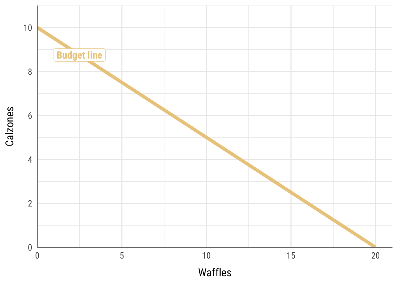
We can write this budget line as an equation following the \(y = mx + b\) format, where \(m\) is the slope and \(b\) is the y-intercept. The slope here is the marginal rate of transformation (MRT).
\[ y = -\frac{1}{2} x + 10 \]
2. Figure out indifference curves and the MRS
We can afford every combination of waffles and calzones along the budget line, but we don’t know what the optimal mix of waffles and calzones is—that depends on how much we like the two foods, or our preferences.
Our utility function is \(u = xy\), which means that we multiply the quantity of waffles and calzones together to get our utility. That is, if we eat 10 waffles and 4 calzones, we’ll get 40 utils; if we eat 5 waffles and 14 calzones, we’ll get 70 utils; and so on.
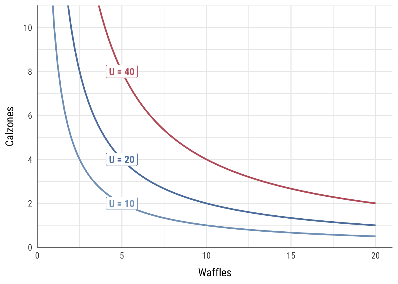
Indifference curves show all the combinations of two goods that provide the same utility. If we want to get 40 utils, we could eat 20 waffles and 2 calzones, 10 waffles and 4 calzones, 5 waffles and 8 calzones, etc. Each of those combinations provides 40 utils of happiness.
We can calculate the combinations of waffles and calzones that lead to any amount of utility. In the chart below, I show three different indifference curves. Every point along the curve represents the combination of waffles and calzones that would lead to 10, 20, and 40 utils.
Next, we can use this utility function to calculate the marginal rate of substitution or MRS, which is the slope of the curve at any given point. In calculus land, we find the slope of a function by calculating the first derivative. For easier one-variable functions like \(x^2\), this involves moving the exponent down, multiplying it by the coefficient, and reducing the exponent by one. The first derivative of \(x^2\) is \(2x\). The derivative of \(2x^3\) would be \(6x^2\), and so on.
When differentiating a two-variable function like \(xy\), though, we can’t just follow the simple rule of moving an exponent down and subtracting one. Instead, we have to calculate partial derivatives—we find the derivative of just the \(x\) part while holding \(y\) constant and divide it by the derivative of just the \(y\) part while holding \(x\) constant.
Don’t worry if that sounds complicated. The easiest way to do this is to go to Wolfram Alpha, type in the phrase “derivative xy” and see what it calculates for you. You’ll see two partial derivatives: \(\frac{\partial}{\partial x}\) and \(\frac{\partial}{\partial y}\). Make those two partial derivatives a ratio and you’ll have the derivative of the whole function: \(\frac{\partial / \partial x}{\partial / \partial y}\). To make your life easier, I will occasionally provide you with the MRS in problem sets or tests.Which I’ll calculate by letting Wolfram Alpha do it for me.
In this case, where \(u = xy\), the slope / first derivative / MRS is \(\frac{y}{x}\).
Next, we can add actual numbers to this MRS by setting it equal to the ratio of the prices of waffles and calzones (remember from that big list of things that MRS is, from up above, that MRS also is \(\frac{\text{Price}_x}{\text{Price}_y}\)):
\[ \frac{y}{x} = \frac{1}{2} \]
We can use algebra to rearrange this formula so that it’s based on \(y\):
\[ y = \frac{1}{2} x \]
That is our MRS given the prices that exist in the world. Phew.
3. Set MRS = MRT and solve for x and y
Now that we have formulas for the MRT and the MRS, we can set them equal to each other to find where they are tangent to each other (i.e where their slopes are the same). Algebra time!
\[ \begin{aligned} MRS &= MRT \\ \frac{1}{2} x &= -\frac{1}{2} x + 10 \\ x &= 10 \end{aligned} \]
The optimal level of waffles is thus 10. We can plug that back into either the MRS or the MRT equation to figure out the optimal level of calzones:
\[ \begin{aligned} y &= -\frac{1}{2} x + 10 \\ y &= (-\frac{1}{2} \times 10) + 10 \\ y &= 5 \end{aligned} \]
5 calzones! The best combination food that maximizes our utility given our budget constraint and current prices is 10 waffles and 5 calzones.
We can use our utility function to calculate how many utils we get from that level of consumption: \(u = xy\), or 10 × 5, or 50.
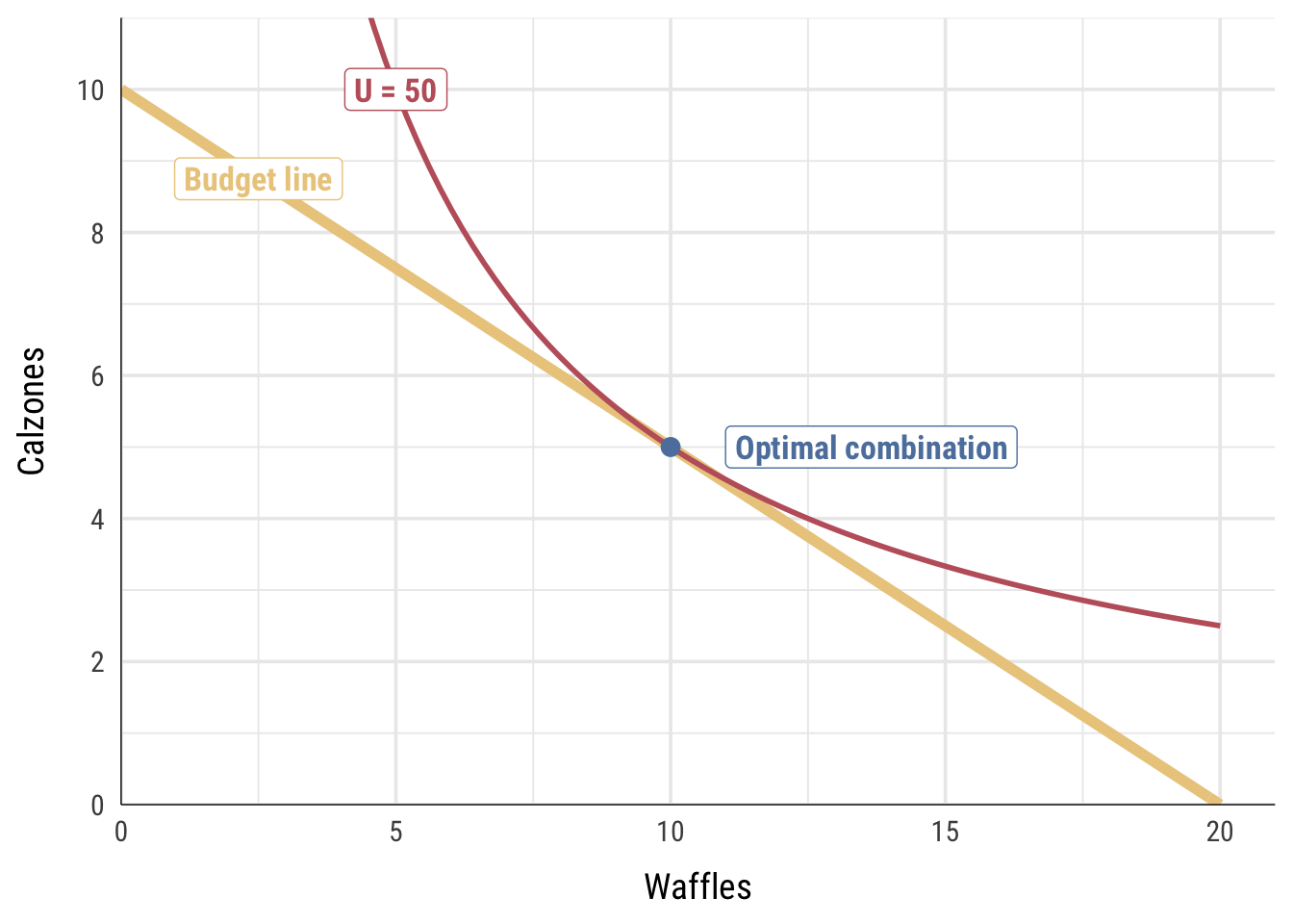
We can verify this combination graphically by plotting the budget line and indifference curve for 50 utils all at the same time:
tl;dr Desmos version
You can avoid some of the math get the same answer by plotting these formulas at Desmos or with a graphing calculator:
- Figure out the budget line or feasible set and plot it: \(y = -\frac{1}{2}x + 10\)
- Figure out the MRS (\(\frac{y}{x}\)), set it equal to the price ratio (\(\frac{1}{2}\)), and rearrange it so that it is in terms of y: \(y = \frac{1}{2} x\). Plot that.
- Notice how the two lines intersect at (10, 5). That’s the optimal point.
- You can add an indifference curve by figuring out what level of utility you get when consuming 10 waffles and 5 calzones (10 × 5), and then plotting the utility function at that level. You don’t need to rearrange the formula or anything; Desmos is smart enough to figure it out: \(50 = xy\).
- If you did it right, you should get an indifference curve tangent to the budget line at (10, 5).
Clearest and muddiest things
Go to this form and answer these three questions:
- What was the muddiest thing from class today? What are you still wondering about?
- What was the clearest thing from class today?
- What was the most exciting thing you learned?
I’ll compile the questions and send out answers after class.