Firms and markets I
Materials for class on Thursday, October 10, 2019
Contents
Slides
Download the slides from today’s class.

Stone cold sober chocolate milk
Finding the cheapest cost of production
Cost function
| Quantity | Milk | Sugar | Chocolate powder | Spoon | Pot | Fridge |
|---|---|---|---|---|---|---|
| $0 | 0 | 0 | 0 | 1 | 4 | 15 |
| $1 | 2 | 0.5 | 0.1 | 1 | 4 | 15 |
| $2 | 6 | 1.5 | 0.3 | 1 | 4 | 15 |
| $3 | 12 | 3 | 0.6 | 1 | 4 | 15 |
| $4 | 20 | 5 | 1 | 1 | 4 | 15 |
| $5 | 30 | 7.5 | 1.5 | 1 | 4 | 15 |
| $6 | 42 | 10.5 | 2.1 | 1 | 4 | 15 |
| $7 | 56 | 14 | 2.8 | 1 | 4 | 15 |
| $8 | 72 | 18 | 3.6 | 1 | 4 | 15 |
| $9 | 90 | 22.5 | 4.5 | 1 | 4 | 15 |
| $10 | 110 | 27.5 | 5.5 | 1 | 4 | 15 |
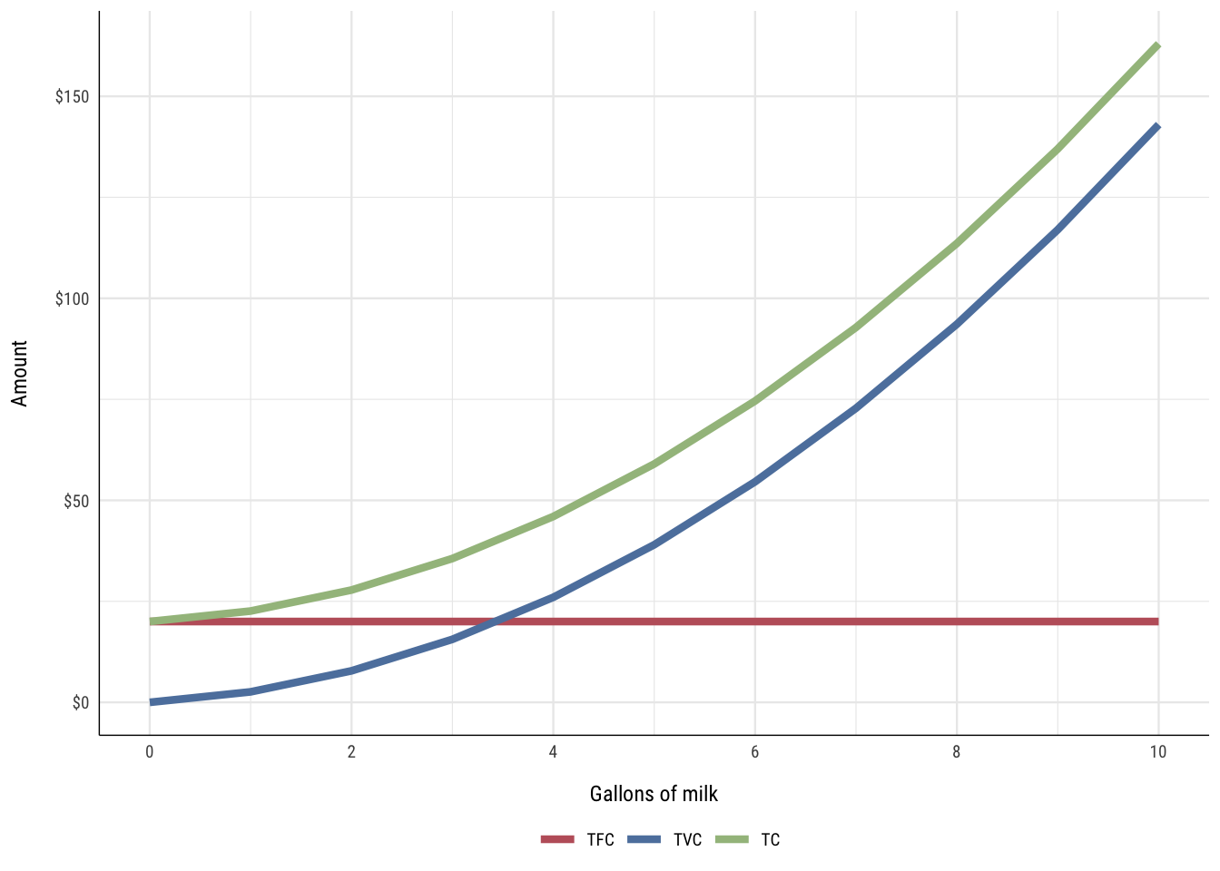
Total costs
| Quantity | TFC | TVC | TC |
|---|---|---|---|
| $0 | 20 | 0 | 20 |
| $1 | 20 | 2.6 | 22.6 |
| $2 | 20 | 7.8 | 27.8 |
| $3 | 20 | 15.6 | 35.6 |
| $4 | 20 | 26 | 46 |
| $5 | 20 | 39 | 59 |
| $6 | 20 | 54.6 | 74.6 |
| $7 | 20 | 72.8 | 92.8 |
| $8 | 20 | 93.6 | 113.6 |
| $9 | 20 | 117 | 137 |
| $10 | 20 | 143 | 163 |
If we decompose total costs into fixed and variable costs, we see that the rise in costs is driven almost entirely by increasing variable costs.
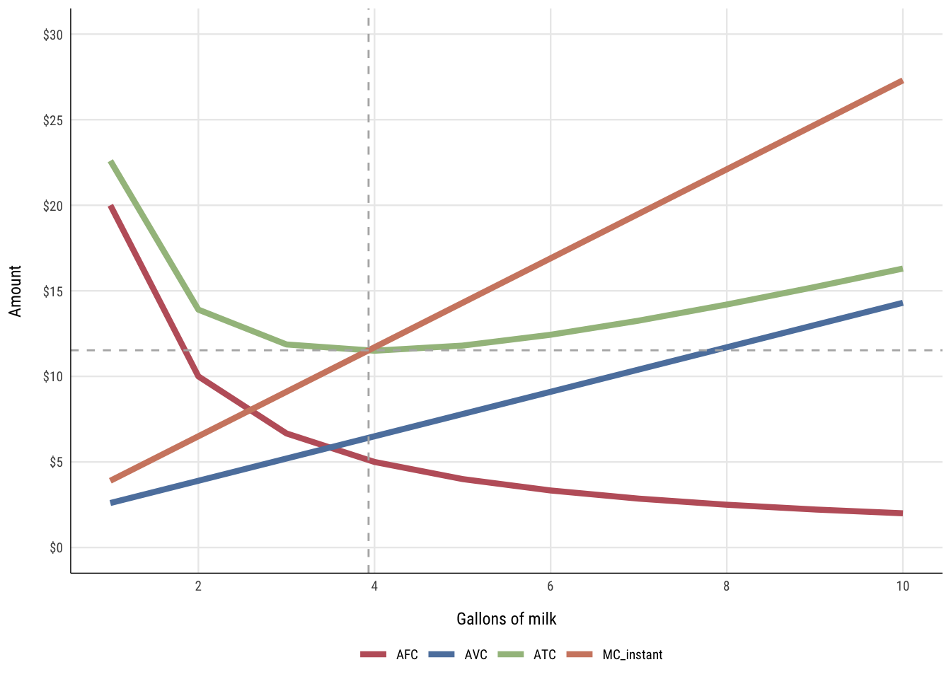
Average costs
| Quantity | TC | AFC | AVC | ATC | MC_chunk | MC_instant |
|---|---|---|---|---|---|---|
| 0 | $20.00 | — | — | — | — | $1.30 |
| 1 | $22.60 | $20 | $2.60 | $22.60 | $2.60 | $3.90 |
| 2 | $27.80 | $10 | $3.90 | $13.90 | $5.20 | $6.50 |
| 3 | $35.60 | $7 | $5.20 | $11.87 | $7.80 | $9.10 |
| 4 | $46.00 | $5 | $6.50 | $11.50 | $10.40 | $11.70 |
| 5 | $59.00 | $4 | $7.80 | $11.80 | $13.00 | $14.30 |
| 6 | $74.60 | $3 | $9.10 | $12.43 | $15.60 | $16.90 |
| 7 | $92.80 | $3 | $10.40 | $13.26 | $18.20 | $19.50 |
| 8 | $113.60 | $2 | $11.70 | $14.20 | $20.80 | $22.10 |
| 9 | $137.00 | $2 | $13.00 | $15.22 | $23.40 | $24.70 |
| 10 | $163.00 | $2 | $14.30 | $16.30 | $26.00 | $27.30 |
The optimal point on the ATC curve occurs when Q = 3.93. This is also not coincidentally where the MC curve intersects the ATC curve. The optimal price at this quantity is $11.52 per gallon of milk, but the firm won’t necessarily be able to set the price at that point on its own (unless it’s a monopoly; and even then, they’ll set it higher).
IMPORTANT NOTE: Because we’re dealing with curves and not lines, calculating marginal values with Excel by subtracting the previous value from the current value will not be 100% accurate. The only way to get perfectly accurate marginal values is to use calculus to find the instantaneous derivative at exactly that point.
Finding the optimal price and quantity
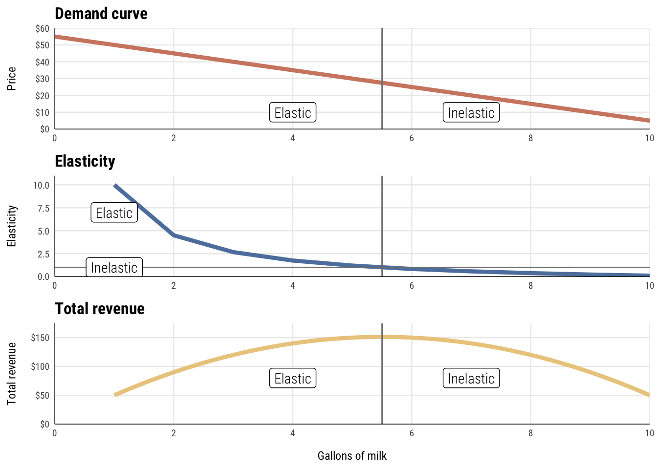
The firm’s quantity decision depends on the market demand for chocolate milk. The demand curve for this market looks like this:
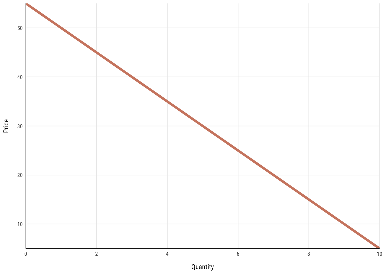
With this demand curve, we can find the price and quantity that would produce the maximum revenue, assuming there were no costs to production.
| Quantity | Price | TR |
|---|---|---|
| 0 | $55 | $0 |
| 1 | $50 | $50 |
| 2 | $45 | $90 |
| 3 | $40 | $120 |
| 4 | $35 | $140 |
| 5 | $30 | $150 |
| 6 | $25 | $150 |
| 7 | $20 | $140 |
| 8 | $15 | $120 |
| 9 | $10 | $90 |
| 10 | $5 | $50 |
The firm can maximize its revenue by producing 5.5 gallons of milk, which would create $151.25 in revenue.
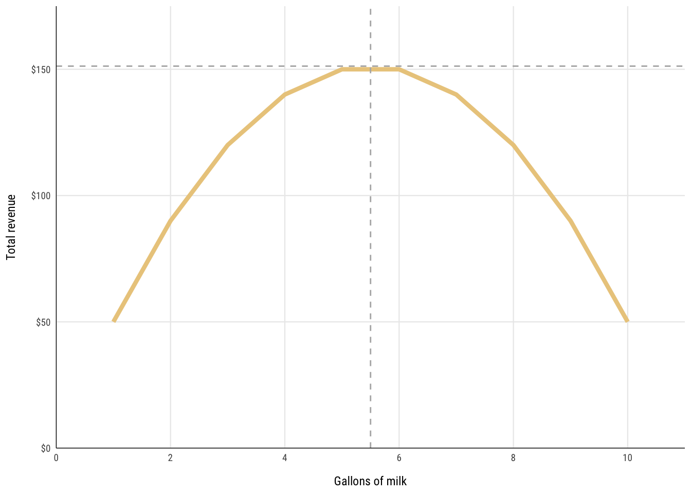
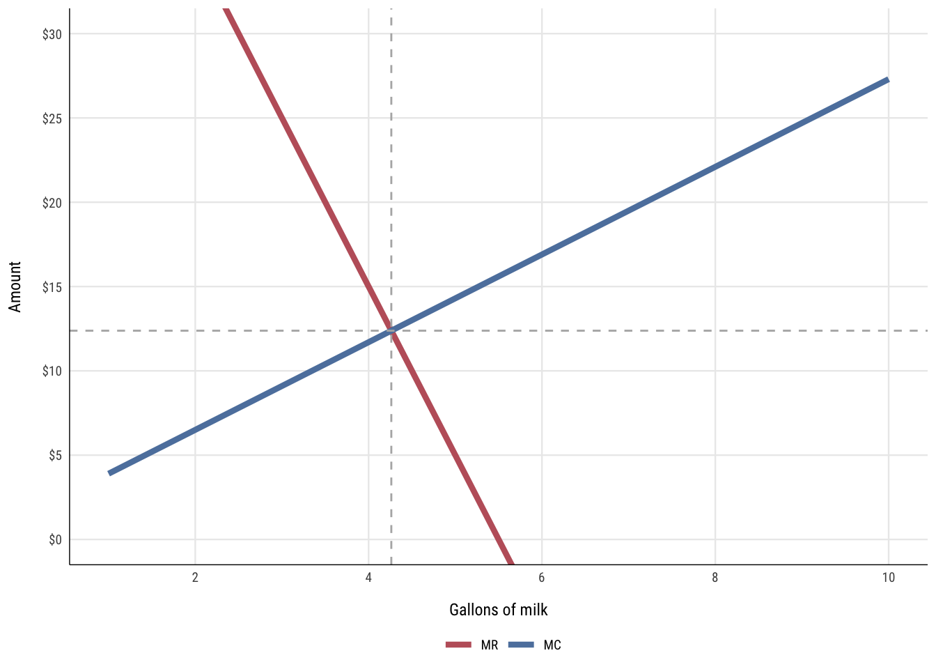
However, this doesn’t take into account the firm’s costs. The firm’s profit maximizing point is defined as \(MC = MR\), so we need compare marginal costs and marginal revenues and calculate total profit (π) across all quantities of output.
Again, note that using chunky marginal values by subtracting previous values won’t be as accurate as calculus-based instant marginal values.
To get correct marginal values we can find the formula for the total cost function by using Wolfram Alpha. If you make a list of all the points in the quantity and total cost columns (i.e. {{0, 20}, {1, 22.6}, {2, 27.8}}), you can fit a polynomial formula to those points with Wolfram Alpha.
For example, search for “quadratic fit {0, 20}, {1, 22.6}, {2, 27.8}, {3, 35.6}, {4, 46}, {5, 59}, {6, 74.6}, {7, 92.8}, {8, 113.6}, {9, 137}, {10, 163}” and you’ll see that the best formula for total cost is \(y = 1.3x^2 + 1.3x + 20\).
The marignal cost is the first derivative of the total cost, or \(y = 2.6x + 1.3\).
To find the equation for total revenue we need to multiply the demand function by Q (or x), since the formula for total revenue is \(TR = PQ\). By looking at the demand curve above, we can see that the y-intercept is 55 and the slope is −5, giving us \(y = -5x + 55\). If we multiple that by x, we get a total revenue formula of \(y = -5x^2 + 55x\) (or \(P = -5Q^2 + 55Q\)).
The marginal revenue is the first derivative of the total revenue, or \(y = -10x + 55\).
We can set MR and MC equal to each other to find the optimal x (or Q) (\(2.6x + 1.3 = -10x + 55\)), solve for x, and then plug that x into one of the total equations to find the optimal price.
The point where \(MC = MR\) can’t be seen in the table, since it happens between 4 and 5 gallons. If the firm produces 4.26 gallons of milk at a price of $12.38 per gallon, it will achieve its maximum profit of $94.43.
| Quantity | Price | TR | TC | MR_chunk | MR_instant | MC_chunk | MC_instant | π |
|---|---|---|---|---|---|---|---|---|
| 0 | $55.00 | $0.00 | $20.00 | — | $55.00 | — | $1.30 | $-20.00 |
| 1 | $50.00 | $50.00 | $22.60 | $50.00 | $45.00 | $2.60 | $3.90 | $27.40 |
| 2 | $45.00 | $90.00 | $27.80 | $40.00 | $35.00 | $5.20 | $6.50 | $62.20 |
| 3 | $40.00 | $120.00 | $35.60 | $30.00 | $25.00 | $7.80 | $9.10 | $84.40 |
| 4 | $35.00 | $140.00 | $46.00 | $20.00 | $15.00 | $10.40 | $11.70 | $94.00 |
| 4.262 | $33.69 | $143.59 | $49.15 | $17.38 | $12.38 | $11.08 | $12.38 | $94.43 |
| 5 | $30.00 | $150.00 | $59.00 | $10.00 | $5.00 | $13.00 | $14.30 | $91.00 |
| 6 | $25.00 | $150.00 | $74.60 | $0.00 | $-5.00 | $15.60 | $16.90 | $75.40 |
| 7 | $20.00 | $140.00 | $92.80 | $-10.00 | $-15.00 | $18.20 | $19.50 | $47.20 |
| 8 | $15.00 | $120.00 | $113.60 | $-20.00 | $-25.00 | $20.80 | $22.10 | $6.40 |
| 9 | $10.00 | $90.00 | $137.00 | $-30.00 | $-35.00 | $23.40 | $24.70 | $-47.00 |
| 10 | $5.00 | $50.00 | $163.00 | $-40.00 | $-45.00 | $26.00 | $27.30 | $-113.00 |
Elasticity of demand
Finally, we calculated the elasticity of demand of chocolate milk. Recall the formula for elasticity:
\[ \begin{align} \varepsilon &= -\frac{\% \text{ change in demand}}{\% \text{ change in price}} \\ &= - \frac{\% \Delta Q}{\% \Delta P} \end{align} \]
Remember that \(\% \Delta Q = \frac{Q_{\text{new}} - Q}{Q}\) and that \(\% \Delta P = \frac{P_{\text{new}} - P}{P}\) (or just \(\frac{\text{new} - \text{old}}{\text{old}}\)). We can also write \(Q_{\text{new}} - Q\) as \(\Delta Q\), or just the change in \(Q\) (and also \(\Delta P\)) This means we can rewrite the equation like so:
\[ \begin{align} \varepsilon &= - \frac{\% \Delta Q}{\% \Delta P} \\ &= - \frac{\frac{Q_{\text{new}} - Q}{Q}}{\frac{P_{\text{new}} - P}{P}} \\ &= - \frac{\frac{\Delta Q}{Q}}{\frac{\Delta P}{P}} \end{align} \]
We can then simplify this huge hairy fraction by multiplying both the numerator and denominator by the inverse of the denominator, \(\frac{P}{\Delta P}\):
\[ \begin{align} \varepsilon &= - \frac{\frac{\Delta Q}{Q}}{\frac{\Delta P}{P}} \times \frac{\frac{P}{\Delta P}}{\frac{P}{\Delta P}} \\ &= - \frac{\Delta Q}{Q} \times \frac{P}{\Delta P} \\ &= - \frac{\Delta Q}{\Delta P} \times \frac{P}{Q} \end{align} \]
That’s the final version of the price elasticity of demand formula: \(\varepsilon = - \frac{\Delta Q}{\Delta P} \times \frac{P}{Q}\). Conveniently, \(\frac{\Delta Q}{\Delta P}\) is also the slope of the demand curve.
| Quantity | Price | \(\frac{\Delta Q}{\Delta P}\) | \(\frac{P}{Q}\) | ε |
|---|---|---|---|---|
| 1 | $50 | -0.2 | 50 | 10 |
| 2 | $45 | -0.2 | 22.5 | 4.5 |
| 3 | $40 | -0.2 | 13.33 | 2.667 |
| 4 | $35 | -0.2 | 8.75 | 1.75 |
| 5 | $30 | -0.2 | 6 | 1.2 |
| 6 | $25 | -0.2 | 4.167 | 0.8333 |
| 7 | $20 | -0.2 | 2.857 | 0.5714 |
| 8 | $15 | -0.2 | 1.875 | 0.375 |
| 9 | $10 | -0.2 | 1.111 | 0.2222 |
| 10 | $5 | -0.2 | 0.5 | 0.1 |
Demand is elastic as long as the slope of the revenue function is positive, and demand is inelastic when the slope of revenue is negative, as seen here:
Clearest and muddiest things
Go to this form and answer these three questions:
- What was the muddiest thing from class today? What are you still wondering about?
- What was the clearest thing from class today?
- What was the most exciting thing you learned?
I’ll compile the questions and send out answers after class.